And if you don’t know, now you know

TL;DR: I made a spicy little benchmark of uncertainty estimation for classification, based mostly on A survey of Uncertainty in Deep Neural Networks¹. Based on this, I’m quite excited about evidential deep learning, which I think can tell the difference between out-of-distribution samples and in-distribution but uninformative samples.

Code is here, I welcome comments, thoughts, ideas, etc. Figures that are taken from elsewhere¹²³⁴⁵ have been marked as such in their captions. Code that was taken from elsewhere is marked directly in the file, in a comment, but I’m mostly grateful to this repo for the EDL implementation.

Skippable background

Recently, I was asked to train a classifier on a problem that I fully expected would be an easy problem. It was a large dataset, a two class problem, and there was a known signal for the positive class. To my surprise, however, the first few tests I ran ended up performing almost exactly randomly. After digging a bit into the data, I realized that although there was a known signal for the positive class, that known signal didn’t appear in all of the positively labelled sampled. In other words, many of the images that I was getting were uninformative.

What was annoying about the network⁶ wasn’t that it was wrong, it was that it was confidently wrong. This struggle got me thinking about ways that I could get my network to just admit when it didn’t know. This prompted a deep⁷ dive into uncertainty estimation. This post describes what I did to think about it.

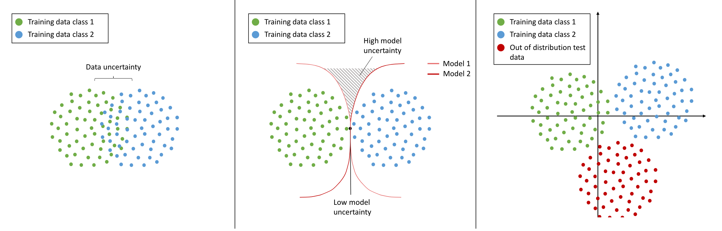
Types of uncertainty

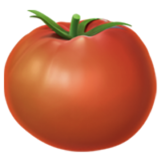
The uncertainty literature seems to distinguish between two types of uncertainties: data (or aleatoric) uncertainty and model (or epistemic) uncertainty. Model uncertainty can usually be fixed with more data.

Out-of-distribution detection is a sub-task related to model uncertainty. When a neural network sees something that it has never seen before, we should not expect it to give a (reasonable) output. This can theoretically be solved with more data, but in practice that would require training with all possible out-of-distribution samples⁸.

Data uncertainty is a harder nut to crack, and was what I thought I was dealing with. It is inherent in the data, so it cannot be fixed with more data. Even though it can’t be fixed, learning to quantify it is immensely eye-opening already. It helps trouble-shoot (is my model not learning at all, or is it learning that there isn’t anything to learn?), filter out points (how confident is this prediction?), and even potentially learn something about the data (namely, its inherent stochasticity).

The data

As anybody who has worked with me long enough will tell you, I usually learn these kinds of concepts by generating a silly synthetic dataset, trying a bunch of techniques as quickly as possible, and accumulating anecdotal evidence and gut feelings. For this project, the task was determining how spicy an image was, based on the amount of pepper in it.

Juicy	Mild	Spicy	OOD

The data was synthetically generated from a set of vegetable templates. I randomly picked a number of each template, scale and rotate them, and put them together onto a plain background. Whichever vegetable is most represented defines the class of the image as a whole.

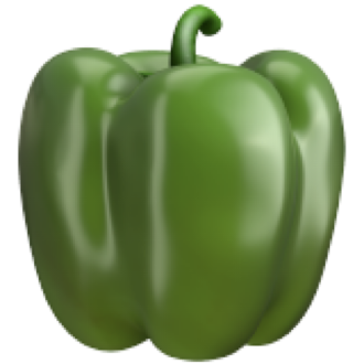
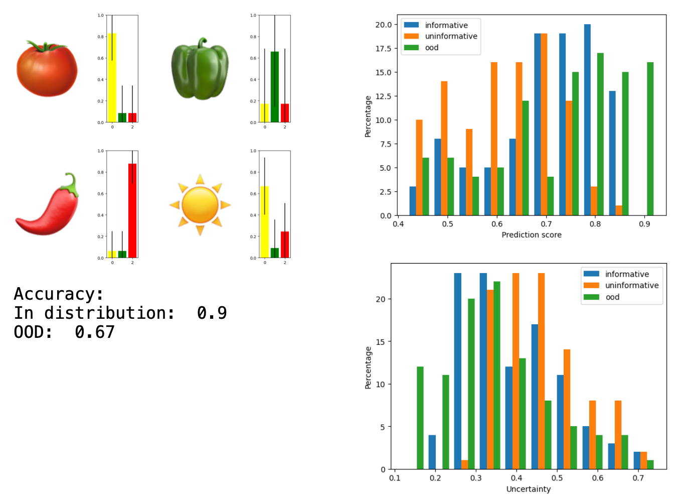
I also created out-of-distribution images by including an emoji in the testing set that was not see in the training set. I chose the sun because the sun is hot, but not necessarily spicy⁹. Images that include the sun are dubbed out-of-distribution¹⁰, but I have made sure that they all have a correct class as well. This way, it makes sense to talk about the accuracy of the network on out-of-distribution examples. Is this a nod to generalization? Perhaps.

Finally, I created uninformative¹¹ samples but choosing two of the vegetables and putting the same number of each in the image. Ideally, this should return a 50/50 split between the two options. The hope, here was that if the model had understood the concept (that the number of items of each type defined the class), then it would output a very low uncertainty for this 50/50 split.

Informative	Juicy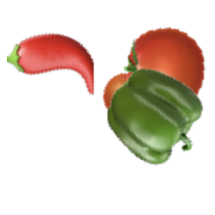	Mild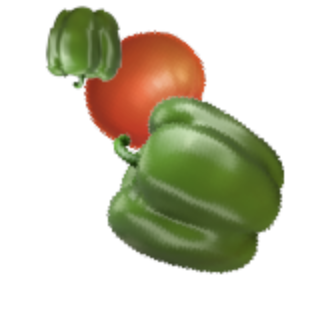	Spicy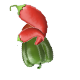
OOD(but informative)	Juicy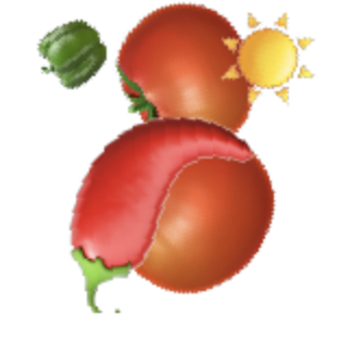	Mild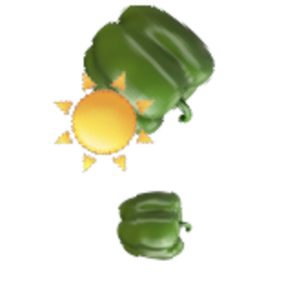	Spicy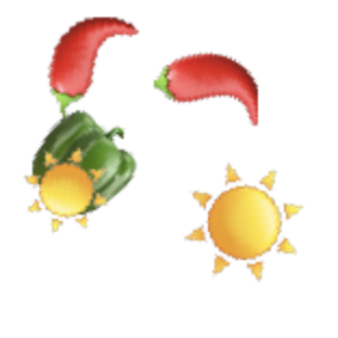
Uninformative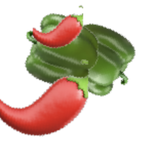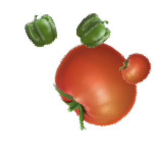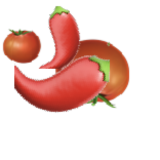

The benchmark

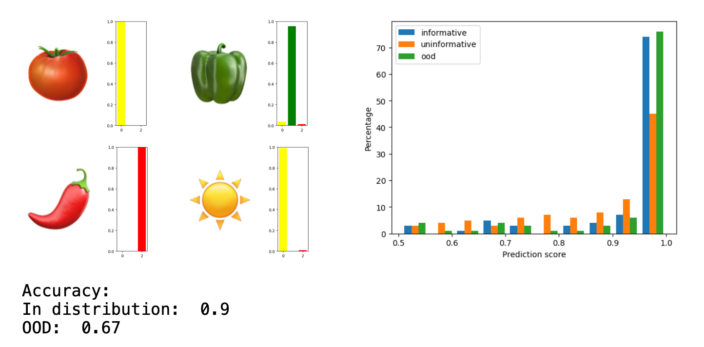
The baseline model that I used was a 3-class VGG, as implemented here

• fmaps=32
• output_classes=3
• input_fmaps=3

I trained for 1000 iterations, with a batch size of 16, with a Cross Entropy loss and an Adam optimizer.

The questions that I wanted to answer each time were:

• How are the templates classified?
• What is the in-distribution vs out-of-distribution accuracy?
• How can I estimate the uncertainties for:
  • informative samples
  • uninformative samples
  • out-of-distribution samples

The hope was to get a high accuracy for both in-distribution and out-of-distribution samples, but with a much higher uncertainty for out-of-distribution samples.

All results will be compared to the baseline below.

The methods

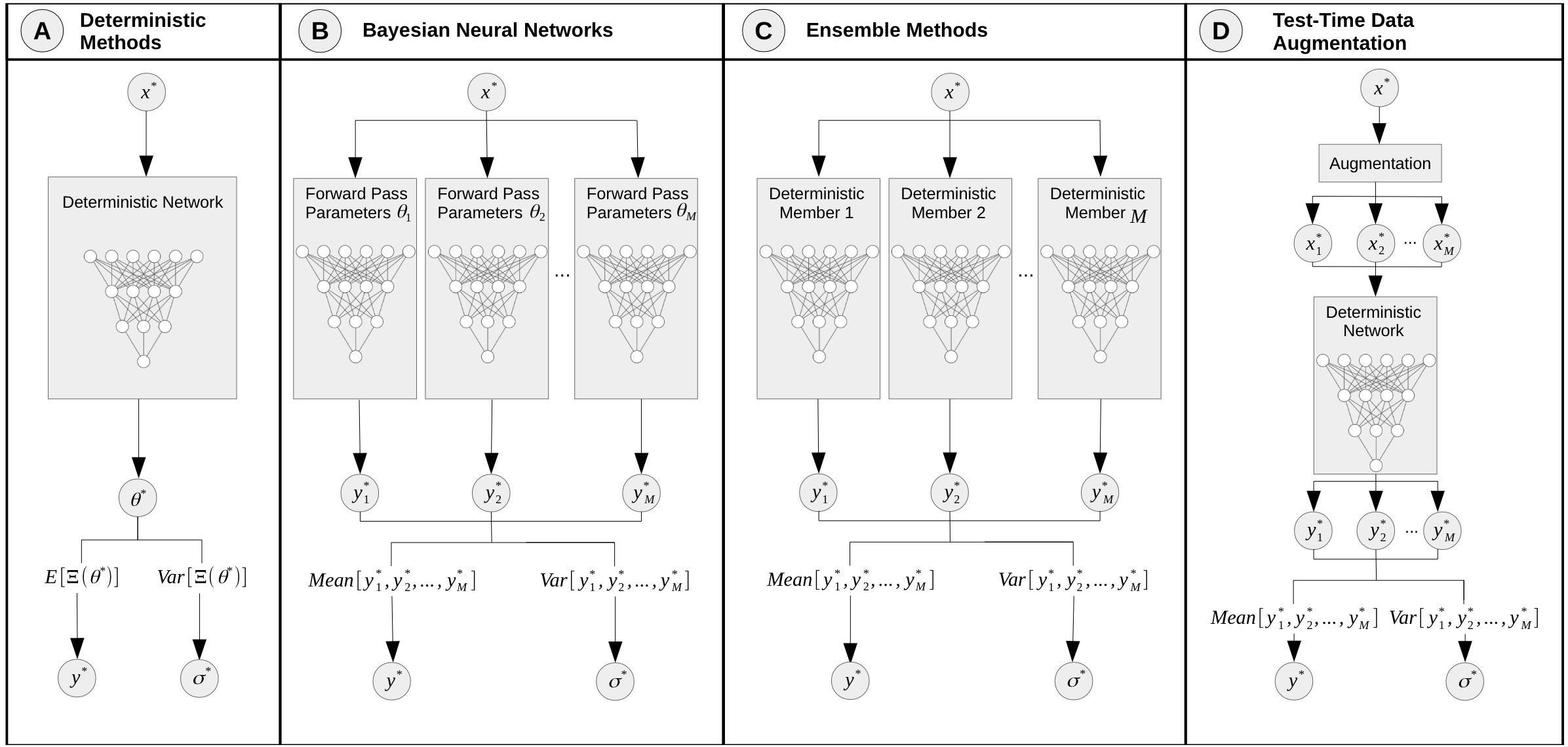
Test-time augmentation

What it does

• Addresses epistemic uncertainty using data augmentation
• No need to re-train
• Augmentations can be user-defined or learned

What I did

• Right-angle rotations and flips
• Mean and std of softmax(logits)

Bayesian method - Dropout

What it does

• Addresses epistemic uncertainty using probabilistic model weights
• Special training necessary

What I did

• Dropout in the dense layers of VGG (test and train)
• 10 forward passes for each sample
• Mean and Std of softmax(logits)

Ensemble method - Random initialization

What it does

• Addresses epistemic uncertainty using a variety model weights
• Special training necessary

What I did

• Trained 10 identical VGG networks on the same data with different random initializations
• Each sample goes through all 10 networks
• Mean and Std of softmax(logits)

Interlude - The Dirichlet distribution

This is the figure that convinced me to fully read the paper.

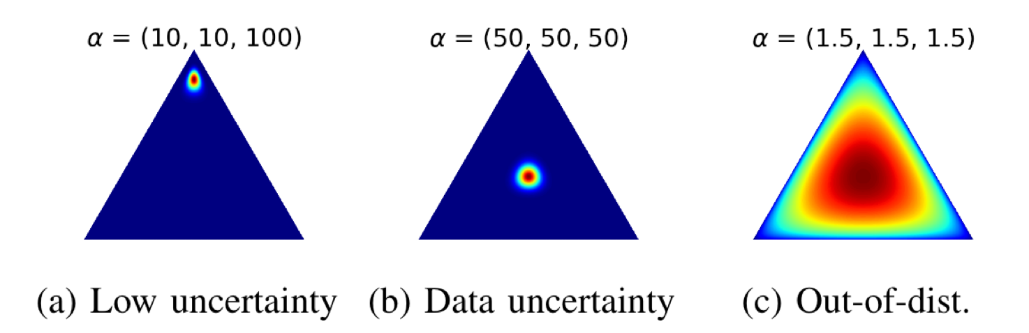
This is a representation of the Dirichlet distribution, which we’ll soon use to create simple classifiers with probabilistic outputs. The Dirichlet distribution for a $K$-category problem is parametrized by values $\alpha_k > 0$. In the context of neural networks consider this:

• each point in the distribution corresponds to a probability distribution over the $K$ classes: this is akin to the output of a classical, softmax-based classifier
• the value of the Dirichlet distribution at that point describes how likely that point is to be “the” output

This is something that confused me for a while, so I’m going to go into a bit more detail about the visualization. The figure in the paper represents a 3-class problem which falls into a 2-simplex as shown below. Each axis represents one of the three variables, which corresponds to the probability of one of the three classes.

(a)

(b)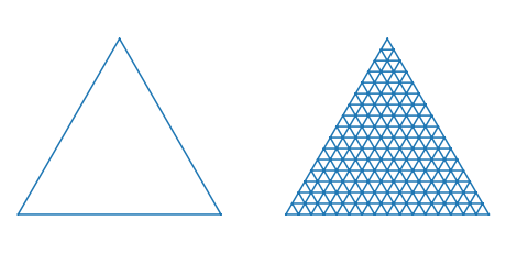

At any point within the triangle, the probabilities sum to one but you have to read the point correctly: taking the axes as parallel to the edges of the triangle.

So if we look at this representation of a Dirichlet distribution from Wikipedia, we can see that the “most likely” output would be approximately: $[x_1 = 0.1 , x_2 = 0.2, x_3 = 0.7]$.

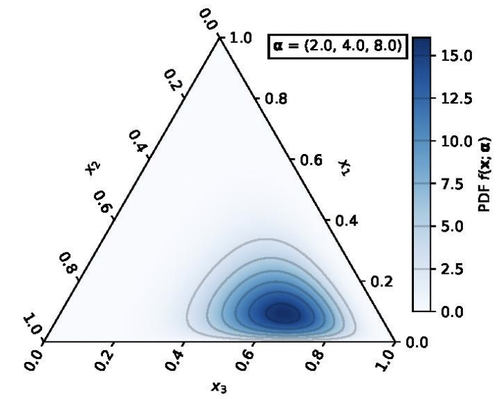
For reference, the distribution is defined as such: \(D_\alpha(\textbf{p}) = \frac{1}{B(\alpha)}\prod_{i=1}^{K} p_{ij}^{\alpha_{ij} - 1}\)

Evidential deep learning

The essence of evidential deep learning (EDL) is to parametrize a belief assignment problem as a Dirichlet distribution and then use a neural network to get the parameters of the distribution.

Belief assignment

In belief assignment, we accumulate evidence $e_i$ for each class. Belief arises as a proportion of total evidence: $b_i = \frac{e_i}{S}$ where \(S =\sum_{i=1}^{K} (ei + 1)\)

The first question that I had when I saw this equation was why is it $e_i + 1$ in the sum? Interestingly, this is where the uncertainty comes up. The whole thing is written up such that we can define the uncertainty as: $u = \frac{K}{S}$. A few interesting this come up from these definitions.

First: if no evidence has been accumulated, then $S = K$ and therefore $u = 1$: we are maximally uncertain. As evidence accumulates, uncertainty grows asymptotically towards zero. I personally like this because it means it never truly reaches zero; we can’t ever truly be sure of something.

Second: we get the nice property of \(u + \sum_{i=1}^{K} b_i = 0\). This leads to the interpretation of the uncertainty as a sort “I don’t know” class. It’s a simplistic interpretation but it was helpful for me to gain intuition.

Bringing back Dirichlet

With a slight re-parametrization of the above, we can turn belief assignment into a Dirichlet distribution. The key is to simply “remove” the troublesome $+1$:

• We define the distribution’s parameters: $\alpha_i = e_i + 1$
• We re-define $S = \sum_{i=1}^{K}\alpha_i$
• We can define probabilities for each class $p_k = \frac{\alpha_k}{S}$
• And $u$ stays defined the same way

With a neural network

The key to training a neural network to give us the $\alpha$ values, is to try to match the expected probabilities with the true labels. I say expected probabilities here deliberately, because we’re going to be integrating over the entire 2-simplex described by the Dirichlet distribution, as described above.

The justification for this in the paper is much more complex, but in the end I simply used an expected mean-squared error as a loss: \(L (\Theta) = \int ||\textbf{y} - \textbf{p}|| D_\alpha(\textbf{p}) d\textbf{p}\)

With:

• $\Theta$ the network parameters
• $D_\alpha$ the Dirichlet distribution
• $\textbf{p}$ the probability vector defined at one point in the distribution, over which we’re integrating.
• $\textbf{y}$ the one-hot encoding of the true class

What I did:

• Replace softmax with a ReLU to get $\alpha$ positive
• Train the network with the loss $L$ above (with an extra annealing step which I won’t get into here)

One thing to note is that this was the most difficult of the networks for me to get running. I had to play around with the parameters of the loss implementation, and run a few examples before I got something accurate. Still, for every other method I am fairly certain that I have reached a good example of a “good-case” scenario¹². For this one, however, I’m sure we can do even better.

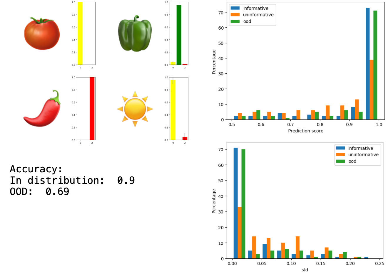
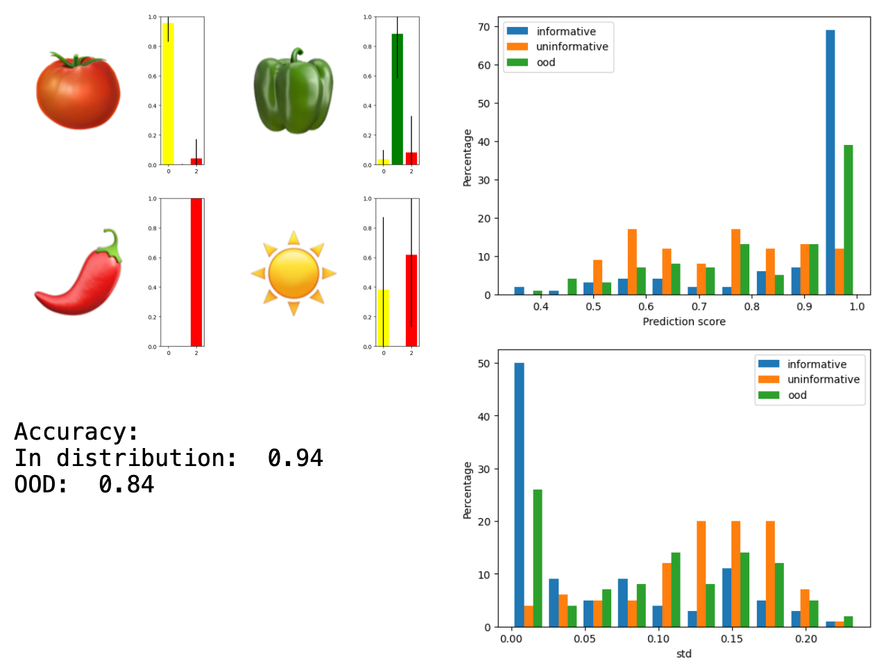
Summary of results

With certain values colored to represent the best example of things we don’t know and of things we know.

Method	In-distribution accuracy	OOD accuracy	In-distribution mean (std) probability	Uninformative mean (std) probability	OOD mean (std) probability	Re-train?	Multi-pass?
Baseline	0.9	0.67	0.94	0.87	0.94	-	-
Test-time augmentation	0.91	0.67	0.93 (0.13)	0.85 (0.15)	0.93(0.14)	No	Yes
MC Dropout	0.9	0.69	0.93 (0.12)	0.87 (0.11)	0.94 (0.14)	Yes	Yes
Ensemble of VGG	0.94	0.84	0.93 (0.13)	0.83 (0.16)	0.91 (0.14)	Yes	Yes
EDL	0.9	0.67	0.71 (0.11)	0.61 (0.1)	0.73 (0.14)	Yes	No

Conclusion

What did I learn? Of all of the methods, the one that I am the most excited about is of course the EDL. I wanted something that is able to tell the difference between uninformative in-distribution samples and out-of-distribution samples, EDL does that. The uninformative in-distribution samples are given lower classification probabilities, but also lower uncertainties: the network is quite certain that there is no information here. In contrast, the out-of-distribution samples are given higher probabilities¹³ but with a higher uncertainty.

Additionally, the EDL just generally shies away from displaying certainty in its probability assignments, which I can’t help but appreciate¹⁴. If we’re going to be using neural networks for science, we need networks whose default is that of a good scientist: complete uncertainty. They need to be able to show when they don’t know and even more importantly when they know that they don’t know.

What I’d want to look at next in the framework of building belief by gathering evidence, is to get a better description of what the evidence is. I don’t like the terms “explainable” or “interpretable” much, but trying to improve our understanding of the “why” of neural networks is most of what I do in my day job. Let’s see what I can find.

References and footnotes